Technique in statistics

Kernel regression

2 min read
In 7 languages

In statistics, kernel regression is a non-parametric technique to estimate the conditional expectation of a random variable. The objective is to find a non-linear relation between a pair of random variables X and Y.

In any nonparametric regression, the conditional expectation of a variable $Y$ relative to a variable $X$ may be written:

\operatorname {E} (Y\mid X)=m(X)

where $m$ is an unknown function.

Nadaraya–Watson kernel regression

Nadaraya and Watson, both in 1964, proposed to estimate $m$ as a locally weighted average, using a kernel as a weighting function. The Nadaraya–Watson estimator is:

{\widehat {m}}_{h}(x)={\frac {\sum _{i=1}^{n}K_{h}(x-x_{i})y_{i}}{\sum _{i=1}^{n}K_{h}(x-x_{i})}}

where $K_{h}(t)={\frac {1}{h}}K\left({\frac {t}{h}}\right)$ is a kernel with a bandwidth $h$ such that $K(\cdot)$ is of order at least 1, that is $\int _{-\infty }^{\infty }uK(u)\,du=0$ .

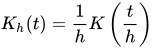
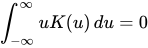
Derivation

Starting with the definition of conditional expectation,

\operatorname {E} (Y\mid X=x)=\int yf(y\mid x)\,dy=\int y{\frac {f(x,y)}{f(x)}}\,dy

we estimate the joint distributions f(x,y) and f(x) using kernel density estimation with a kernel K:

{\hat {f}}(x,y)={\frac {1}{n}}\sum _{i=1}^{n}K_{h}(x-x_{i})K_{h}(y-y_{i}),

{\hat {f}}(x)={\frac {1}{n}}\sum _{i=1}^{n}K_{h}(x-x_{i}),

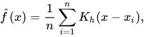
We get:

{\begin{aligned}\operatorname {\hat {E}} (Y\mid X=x)&=\int y{\frac {{\hat {f}}(x,y)}{{\hat {f}}(x)}}\,dy,\\[6pt]&=\int y{\frac {\sum _{i=1}^{n}K_{h}(x-x_{i})K_{h}(y-y_{i})}{\sum _{j=1}^{n}K_{h}(x-x_{j})}}\,dy,\\[6pt]&={\frac {\sum _{i=1}^{n}K_{h}(x-x_{i})\int y\,K_{h}(y-y_{i})\,dy}{\sum _{j=1}^{n}K_{h}(x-x_{j})}},\\[6pt]&={\frac {\sum _{i=1}^{n}K_{h}(x-x_{i})y_{i}}{\sum _{j=1}^{n}K_{h}(x-x_{j})}},\end{aligned}}

which is the Nadaraya–Watson estimator.

Priestley–Chao kernel estimator

{\widehat {m}}_{PC}(x)=h^{-1}\sum _{i=2}^{n}(x_{i}-x_{i-1})K\left({\frac {x-x_{i}}{h}}\right)y_{i}

where $h$ is the bandwidth (or smoothing parameter).

Example

This example is based upon Canadian cross-section wage data consisting of a random sample taken from the 1971 Canadian Census Public Use Tapes for male individuals having common education (grade 13). There are 205 observations in total.

The figure to the right shows the estimated regression function using a second order Gaussian kernel along with asymptotic variability bounds.

Script for example

The following commands of the R programming language use the npreg() function to deliver optimal smoothing and to create the figure given above. These commands can be entered at the command prompt via cut and paste.

install.packages("np")
library(np) # non parametric library
data(cps71)
attach(cps71)

m <- npreg(logwage~age)

plot(m, plot.errors.method="asymptotic",
     plot.errors.style="band",
     ylim=c(11, 15.2))

points(age, logwage, cex=.25)
detach(cps71)

Statistical implementation

GNU Octave mathematical program package
Julia: KernelEstimator.jl
MATLAB: A free MATLAB toolbox with implementation of kernel regression, kernel density estimation, kernel estimation of hazard function and many others is available on these pages (this toolbox is a part of the book).
Python: the KernelReg class for mixed data types in the statsmodels.nonparametric sub-package (includes other kernel density related classes), the package kernel_regression as an extension of scikit-learn (inefficient memory-wise, useful only for small datasets)
R: the function npreg of the np package can perform kernel regression.
Stata: npregress, kernreg2

In 7 languages

English català Deutsch 日本語 русский українська 中文

Text from Wikipedia, CC BY-SA 4.0 · Source article